Example from Science

Below is the code to reproduce Figure 4 of Crozier et. al. (2025)

import detectda as dtda
import matplotlib.pyplot as plt
import numpy as np
from skimage import io, transform
import shapely

Upload video and configure polygonal region

The file “Extract 1 of PtCeO2_030303_CO_75fps_1650kx_2116pm_P2_udvd_mf.tif” can be found by downloading “Figure 4.zip” from Zenodo.

# This is the video from Zenodo
vid = io.imread("Extract 1 of PtCeO2_030303_CO_75fps_1650kx_2116pm_P2_udvd_mf.tif")
crop_vid = vid[:, 13:378, 33:312]
polygon = shapely.Polygon(np.array([[219., 354.],
       [157., 350.],
       [ 85., 329.],
       [ 37., 272.],
       [ 10., 188.],
       [ 17.,  95.],
       [ 57.,  44.],
       [167.,  16.],
       [244.,  10.],
       [269.,  27.],
       [249., 163.],
       [229., 321.],
       [217., 355.],
       [219., 354.]]))

Reproduce Figure 4 plot

First we calculate the 0-dimensional cubical persistent homology for each image in the denoised video. Then we calculate the ALPS statistic for each image with dtda_vid.get_alps().

dtda_vid = dtda.ImageSeries(video=crop_vid, polygon=polygon, n_jobs=8)
dtda_vid.fit(sigma=2)
dtda_vid.get_alps()

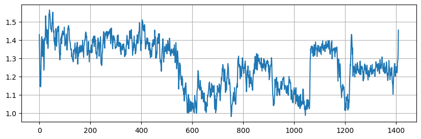
Finally, we employ the standardized ALPS statistic from the Supplementary Material of Crozier et. al. (2025), then plot it to reproduce the figure.

plt.subplots(figsize=(10, 3))

# The standardized ALPS statistic from the Supplementary Material of Crozier et. al. (2025)
std_alps = (dtda_vid.alps + 5.08)/(0.705 * np.log(np.prod(crop_vid.shape[1:])))
plt.plot(std_alps)
plt.grid(axis='both')