Example `detecTDA` usage

In the below, test_video.pkl is the output of the “identify_polygon” python script,
which allows choose your desired polygonal subregion. The video has been preprocessed so each frame is the sum of disjoint blocks of 16 consecutive frames in the original video[1].

import detectda as dtda
import pickle
import matplotlib.pyplot as plt
impol = dtda.ImageSeriesPickle('detectda/tests/test_video.pkl', div=32, n_jobs=2)

Tip

Here we divide each pixel by 32 (div=32) and round to the nearest integer because of various properties of the detector which captured the video. Outside of hypothesis testing context, it is fine to set div equal to its default value of div=1.

Calculate persistent homology

Fit the persistence diagrams for every image in the polygonal region of the test video. We chose a smoothing parameter of 4 worked well for this very noisy nanoparticle video.

impol.fit(sigma=4)

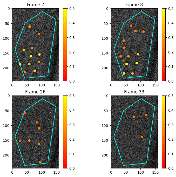
Visualize the results of the fit

See where the persistence features are located and what their lifetimes are. Below, we see a few images with the points of the 0^th persistence diagram overlaid, after removing points with lifetimes less than thr.

plt.figure(figsize=(9, 8))
fs = [6,7,25,32]
for i in range(4):
    plt.subplot(2, 2, i+1)
    plt.title("Frame "+str(fs[i]+1))
    impol.plot_im(fs[i], smooth=False, thr=0.2, vmin=0, vmax=0.5)

png

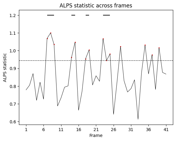
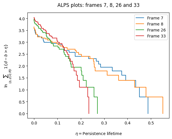
Calculate and plot summaries

Run the get_alps method to calculate the ALPS statistic for each frame (cf. ALPS statistic calculation in the “Example from Science”). We can visualize the ALPS statistic with the following ALPS plot[2], to see how the persistence lifetimes are distributed.

impol.get_alps()
impol.alps_plot([6,7,25,32])

png

Hypothesis testing and plotting

First, we load the video corresponding to the pixels in the vacuum region of the video.

G = open('detectda/tests/test_video_vacuum.pkl', 'rb')
tv_vacuum = pickle.load(G)['video']

Then, we run the hypothesis testing method described in Section 5.3 of Thomas et al. (2023) using the observed image series above, by generating 499 Monte Carlo noise images.

impol_vac = dtda.VacuumSeries(tv_vacuum, observed_ImageSeries=impol, div=32, n_jobs=4)
impol_vac.fit(convert_to_int=True)
impol_vac.transform(499, "alps")

Finally, we plot the results of the hypothesis testing. The original image series consists of 656 frames, and the output here indicates there are quite a few 16-frame blocks with significant topological signal.

impol_vac.plot_hypo()

png

Example detecTDA usage